
Skip to content

Semantic segmentation

Semantic Segmentation Services

Every pixel assigned to a class, and every class turned into a number you can use: area, share, count and change, across street, aerial, industrial and medical imagery.

Sample project · semantic segmentation of a street-level image into classes

Overview

A mask is only useful if you can count something with it

Semantic segmentation assigns every pixel in an image to a class: road, building, vegetation, sky, defect, tissue, crop. What makes it worth doing is the step after that. A mask on its own is a picture; the deliverable is the table it produces — how much of this image is vegetation, how large is this defect in millimetres, how many hectares of this field are under one crop, how did all of that change between two dates.

Which model to use is the least interesting decision, and we make it last. It follows from the imagery and the classes you need: an urban-scene model for street-level views, a remote-sensing model for aerial and satellite tiles, an anomaly model for industrial surfaces, a medical model for CT, MRI and endoscopy. We work from established open architectures rather than building from scratch, because on ordinary projects a proven model with well-prepared data beats a novel model with rushed data every time.

The part that decides whether the numbers hold up is the class definition and the validation. We agree what counts as each class before annotation starts, hand-score a held-out sample after inference, and deliver per-class IoU alongside the results. An unvalidated mask is an opinion rendered in colour.

Real output

Segmentation across four kinds of imagery

The same pipeline shape — define classes, segment, measure, validate — applied to four domains that share almost nothing else. Output below is from established open models on public demonstration data.

Street and driving scenes

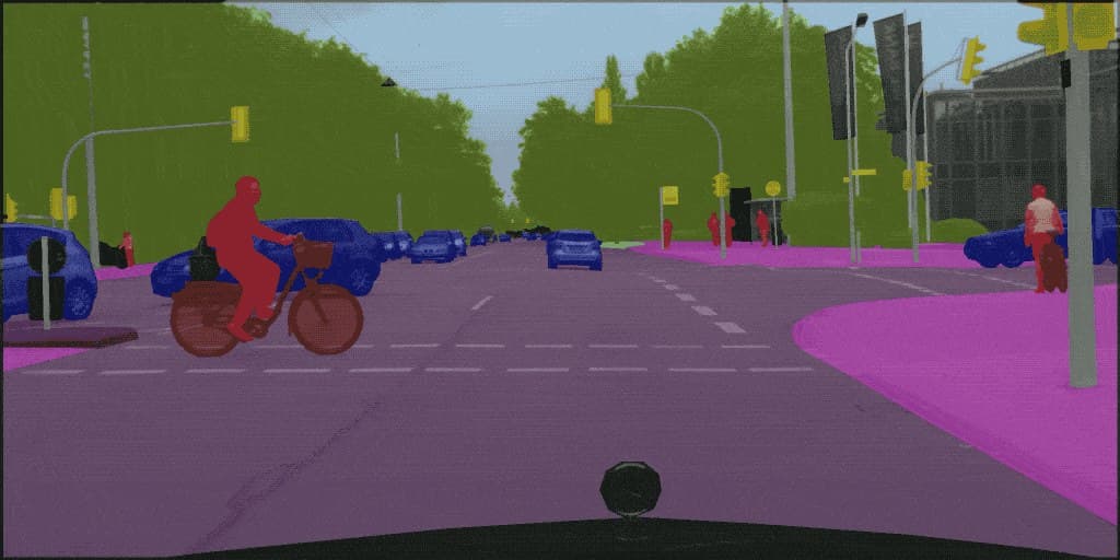
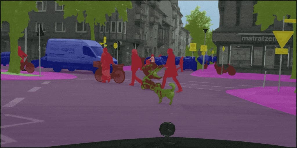
Road, sidewalk, building, vegetation, sky, vehicle and person separated in a single pass. Class shares from images like these become street-level indicators: how green a street reads, how enclosed it feels, how much of the frontage is active.

Street scene 1 with semantic segmentation overlaid, each region coloured by its class
Urban scene
Street scene 2 with semantic segmentation overlaid, each region coloured by its class
Urban scene

Industrial surfaces and defects

Left to right: the input image, the ground-truth annotation, the predicted anomaly heat map, the binary mask and the final outline. Segmentation rather than classification is what makes a defect measurable — its area, its shape and whether it crosses a tolerance.

Five-panel industrial defect segmentation: input image, ground truth, predicted heat map, predicted mask and segmentation result
Defect

Medical imaging

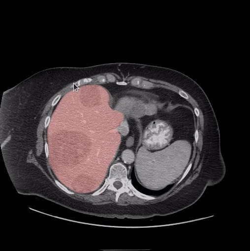
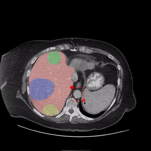
Organs and regions of interest delineated on CT slices. The clinical question is never the mask itself but what follows from it: volume, boundary and change between two scans.

CT slice 1 with organ regions segmented and colour-coded
Medical
CT slice 2 with organ regions segmented and colour-coded
Medical

Aerial and satellite imagery

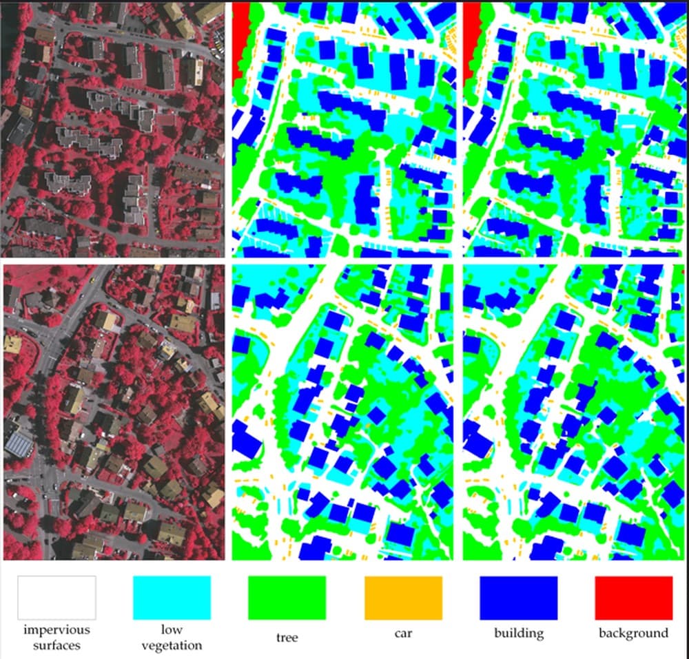
Input tile, reference annotation and prediction side by side, with the class legend below: impervious surface, low vegetation, tree, car, building. Once georeferenced, each class becomes an area you can measure and compare between dates.

Aerial imagery tiles with land-cover segmentation results and a class legend covering impervious surfaces, low vegetation, tree, car, building and background
Aerial

Demonstration imagery from open-source projects, used under their licences: MMSegmentation and Anomalib (Apache-2.0), MedSAM (Apache-2.0) and GeoSeg (GPL-3.0). Shown to illustrate what each class of output looks like; project work is run on your imagery.

Scope

What you receive

Masks are the intermediate product. The statistics derived from them, and the evidence that they are trustworthy, are the deliverable.

  • Per-image masks

    Indexed PNG or single-band GeoTIFF, one value per class, at the resolution of the source image.

  • Class colour map

    The palette and its class mapping as data, so masks render identically wherever they are opened.

  • Per-class statistics

    Pixel count, area and share per class per image, in real units where the imagery is georeferenced or calibrated.

  • Vector polygons

    Masks converted to simplified polygons with a tolerance you choose, for GIS and CAD workflows.

  • Object instances

    Where the question is 'how many' rather than 'how much', connected regions counted and measured individually.

  • Confidence layer

    Per-pixel confidence written alongside the mask, so low-certainty regions can be reviewed rather than trusted blindly.

  • Accuracy report

    Overall and per-class IoU, precision and recall against a manually scored sample, with the sample included.

  • Change comparison

    Where two dates exist, per-class gain and loss between them, with the pairing method stated.

  • Method record

    Model, weights, training or fine-tuning data, thresholds and post-processing, written down and versioned.

  • Inference package

    Optional: the weights and a runnable script, so you can process new imagery yourself afterwards.

Output formats

Delivered the way your stack expects

PNG / TIFF masks
Indexed masks plus optional colour-rendered overlays for review and reporting.
GeoTIFF
Georeferenced masks aligned to the source imagery, ready for QGIS and ArcGIS.
GeoJSON / Shapefile
Vectorised classes with per-polygon area and class attributes.
COCO JSON
Standard annotation format when the output feeds another training pipeline.
CSV / Excel
Per-image and aggregated class statistics with the accuracy report as a separate sheet.
Model weights
ONNX or framework-native weights when the engagement includes handing the model over.

Sample dataset

What you actually receive

Sample project data. Small, thin classes such as people and poles always score lower than large contiguous ones; reporting them separately is the point, because an averaged figure hides exactly the classes most likely to be wrong.

Sample project · Per-class accuracy on a held-out validation set
ClassPixel share %IoUPrecisionRecallSamples
Road surface31.40.940.960.97480
Building24.80.910.930.95480
Vegetation18.20.890.920.94480
Sky12.60.970.980.99480
Vehicle7.10.830.880.90480
Person1.40.680.790.76480

Delivered work

This service on a real project

Sample projects built on this service, with the numbers they produced and what each one settled.

GIS AnalysisComputer VisionMap Visualization

Street Scene Analysis

Measuring the physical character of streets at scale using semantic segmentation, object detection and colour analysis on street-level imagery.

Network analysed
310 km
Images processed
24,800
Indicators per segment
7

What it showed

  • Green view index across the network ranged from 4.1% to 38.9%, and the distribution followed district boundaries far more closely than the team expected. Two adjacent districts differed by more than twenty points with no change in street type.
  • Enclosure ratio and green view were only weakly related. Several streets scored well on greenery while feeling open and exposed, which matters because those two qualities are often treated as one in streetscape policy.
Read the full case study

How it works

Five steps, every project

  1. Step 01

    Tell us what data you need

    The imagery you hold or need collected, the classes that matter and the measurement the result has to support.

  2. Step 02

    We define the data scope

    Class definitions agreed in writing, including the edge cases, plus the accuracy target and how it will be checked.

  3. Step 03

    We collect and process the data

    Annotation where required, model selection and fine-tuning, then inference across the full set.

  4. Step 04

    We validate the dataset

    A held-out sample is scored by hand and compared class by class before anything is delivered.

  5. Step 05

    We deliver the final result

    Masks, statistics, vectors, the accuracy report and the method record — plus weights if the scope includes them.

Projects are priced on image count, whether custom annotation is needed, the number of classes and whether model weights are handed over. Send us a sample of your imagery and the classes you need, and you get a fixed price against a written scope.

FAQ

Questions we get asked

What is semantic segmentation?

It is the assignment of every pixel in an image to a class, as opposed to classification, which labels the whole image, and detection, which draws a box around an object. Segmentation is the right tool when the answer is an area or a shape — how much of this scene is vegetation, what is the extent of this defect — rather than a yes or no.

What imagery can you work with?

Street-level and 360 panoramas, drone and aerial photography, satellite tiles, industrial inspection images, video frames, and medical imaging such as CT, MRI, ultrasound and endoscopy. The practical constraints are resolution relative to the smallest class you care about, and whether the classes are actually visible in the imagery you have.

Do we need annotated training data?

Often not. For common class sets — urban scenes, land cover, standard defect types — pre-trained models transfer well and we validate rather than retrain. Custom classes usually need a few hundred annotated images; we can produce those annotations, or quality-check ones you already have. We tell you which case you are in after looking at a sample, before you commit.

How accurate is it?

It depends on the class, which is why we report per class rather than as one headline number. Large contiguous classes such as road, building and sky typically reach 0.90 or better IoU; small or thin classes such as people, poles and wires sit lower. Every project is validated against a hand-scored sample, and that sample is delivered with the results so you can audit the claim.

Can we run the model ourselves afterwards?

Yes, if that is in scope. We hand over weights, an inference script and the pre- and post-processing steps, so new imagery can be processed in house. Note the licence of the underlying architecture: most are permissive, but some open models carry copyleft terms that affect redistribution, and we flag which applies before work starts.

Can you process video rather than stills?

Yes. Video is sampled to frames at an interval that suits the question, segmented frame by frame, and optionally smoothed across time so a class does not flicker between adjacent frames. Results can be reported per frame, per second or aggregated across a whole clip.

Next step

Have a specific data requirement?

Tell us the geography, the fields and the cadence you need for semantic segmentation. You get a scoped plan, a sample and a fixed price before any work starts.